LeWorldModel: Stable End-to-End JEPA from Pixels
8 min read
Learn what an action changes in a compact latent space. Keep that space from collapsing, then search for actions that bring the predicted future closer to a goal image.
The architecture
Two transformers learn a world that a planner can use
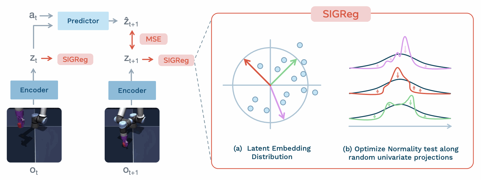
A Joint-Embedding Predictive Architecture (JEPA) predicts future representations. LeWM trains on offline image-action trajectories without reward labels, physical-state labels, or pixel reconstruction.
1. Observe
Encode the image
A ViT-Tiny turns each RGB frame into one 192-dimensional embedding using its final [CLS] token and a projection head.
zₜ = encoder(oₜ)
12 layers · 3 heads · about 5M parameters
2. Imagine
Predict the next latent
A causal transformer reads a short embedding history. Actions condition its layers through Adaptive Layer Normalization (AdaLN).
ẑₜ₊₁ = predictor(z history, aₜ)
6 layers · 16 heads · about 10M parameters
3. Learn
Match the observed future
Encode the actual next frame with the same encoder. Minimize prediction error while SIGReg keeps the embeddings diverse.
L = ‖ẑₜ₊₁ − zₜ₊₁‖² + λ SIGReg(Z)
Both networks learn jointly from pixels and actions
Simplified training flow from Section 3.1. The default model has about 15M parameters. Its predictor uses temporal causal masking; its targets remain connected to the encoder through the prediction loss.
The mental model
Imagine a robot pushing a cube. A policy chooses a push. LeWM predicts the consequence of a proposed push, so a separate optimizer can compare possible plans before executing one. Its output is a future embedding, rather than an action sequence or a rendered video.
Both parts are transformers: a small vision encoder and an action-conditioned dynamics predictor. The predictor uses continuous image embeddings and actions to forecast the next latent state. A decoder can be trained afterward to visualize those states, but reconstruction is outside the world model's training objective and planning loop.
Why prediction alone collapses
The next-frame target is also produced by a trainable encoder. If every image becomes the same vector, the predictor can output that vector for every action. Prediction error reaches zero while the representation loses all useful distinctions.
LeWM adopts the Sketched-Isotropic-Gaussian Regularizer (SIGReg) from LeJEPA. Across observations, it encourages embeddings to follow an isotropic Gaussian distribution, with zero mean and unit variance along each unit direction. A constant embedding cannot satisfy that objective. Individual images still have deterministic embeddings; the distribution constraint applies across examples.
Checking a full high-dimensional distribution is expensive. SIGReg projects a batch of embeddings onto random unit directions, applies an Epps–Pulley test against a standard Gaussian to each projection, and averages the discrepancies. The Cramér–Wold theorem motivates this: matching every one-dimensional projection would match the joint distribution. Finite random projections approximate that goal.
Prediction preserves predictable structure.
SIGReg prevents the constant-vector shortcut.
The default settings are 1,024 projections and λ = 0.1. The paper's single effective tuning parameter refers to the loss weight λ; architecture and training settings still exist. Gradients update both networks, including the target encoder path, without stop-gradient, an exponential-moving-average target encoder, or pretrained features.
How latent predictions become actions
Encode the current image and a goal image. Roll each candidate action sequence forward through the predictor, then score the squared distance between its final predicted embedding and the goal embedding. The model stays fixed throughout this search.
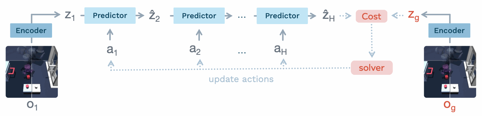
- Sample candidate plans with the Cross-Entropy Method (CEM).
- Keep the lowest-cost plans and refit the sampling distribution.
- Repeat the search, execute the chosen actions, observe again, and replan.
This is model predictive control. In the reported setup, all five planned model steps are executed before replanning. Each step groups five environment actions, so a plan spans 25 environment timesteps. A goal image supplies the objective without a learned reward head.
What changes from DINO-WM and Dreamer?
DINO-WM freezes a pretrained DINOv2 encoder and learns dynamics over its features. The dynamics loss cannot make that fixed encoder collapse, but it also cannot adapt the visual representation to the environment. LeWM learns the representation and dynamics together, with SIGReg supplying the anti-collapse constraint.
DreamerV3 uses reconstruction and prediction objectives to retain information, with KL balancing and free bits regulating its latent posterior and prior. It trains an actor through imagined experience. LeWM instead searches for actions at inference time. The separate Dreamer 4 note covers the later scalable video-model approach.
What do the physical probes tell us?
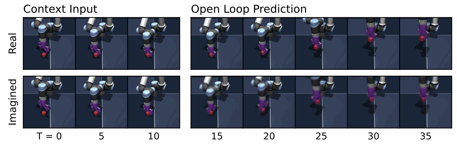
After world-model training, a probe learns to recover a physical quantity from an embedding using simulator labels. A linear probe computes Wz + b; an MLP can recover nonlinear relationships. These labels evaluate the representation rather than supervise the original world-model objective. A hypothetical 192D-to-3D linear position probe needs only 579 parameters, including its bias.
On OGBench-Cube, block position is easy to recover: Pearson correlation is 0.997 for the linear probe and 0.999 for the MLP. Block yaw is much harder, at 0.062 and 0.164 respectively (Appendix F.2, Table 4). Low scores can reflect missing information or information the tested probes cannot decode. Recovering the current position also does not establish accurate future position prediction.
A second test measures surprise as prediction error. Teleporting objects produces stronger surprise than changing their color in the tested environments. That is evidence of learned physical regularity within these tests, rather than a general guarantee of physical reasoning.
Efficient planning, with a compact representation tradeoff
The paper reports up to 48× faster planning than DINO-WM in its comparison, with LeWM completing a plan in under a second. Its compact representation makes candidate rollouts cheaper. Control is competitive across four simulated environments: LeWM leads the compared world models on Push-T and Reacher, while DINO-WM performs better on OGBench-Cube and Two-Room.
These are short-horizon simulation results, not a physical-robot deployment. Goals come from future observations in offline trajectories, and errors accumulate during autoregressive rollouts. Preventing collapse does not ensure that every variable needed for a later task survives compression. The useful contribution is a simple way to learn non-collapsing latent dynamics directly from pixels, while leaving that representation tradeoff visible.
Sources