Robot Control and Markov Decision Processes
Notes from Lecture 2 of Robot Learning: From Fundamentals to Foundation Models, taught by Oier Mees.
Robot control is the bridge from a high-level goal to physical motion: geometry tells us where the robot can move, controllers make motion happen, and MDPs give learning algorithms a clean decision-making language.
Different robots still share one control problem
A quadruped, a dexterous hand, a drone, and a robot arm look completely different.
But the core problem is the same: convert some high-level goal into motor commands that move that robot's particular body through the world.
That is why control foundations come before learning. If we want general robot learning, we need a common language for very different morphologies.
Rigid bodies give robotics a common language
Most robot parts can be approximated as rigid bodies.
Rigid means the object can translate and rotate, but points on the object do not stretch or squish relative to each other.
This matters because we do not need to track every point separately. We can describe the body by a pose: where it is and how it is oriented.
Any robot morphology can be represented as a rigid body moving through the space.
SE(2) and SE(3) describe pose without deforming the robot
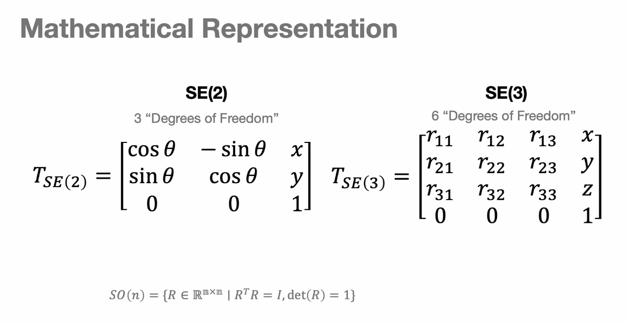
For planar motion, like a ground robot, pose lives in SE(2): x, y, and heading.
For full 3D motion, like a drone or robot hand in space, pose lives in SE(3): translation plus roll, pitch, and yaw.
The rotation part must stay a valid rotation matrix: orthogonal, with determinant 1. That keeps rotation from accidentally becoming stretching or shearing.
Homogeneous transforms let frames talk to each other
A robot rarely has one coordinate frame.
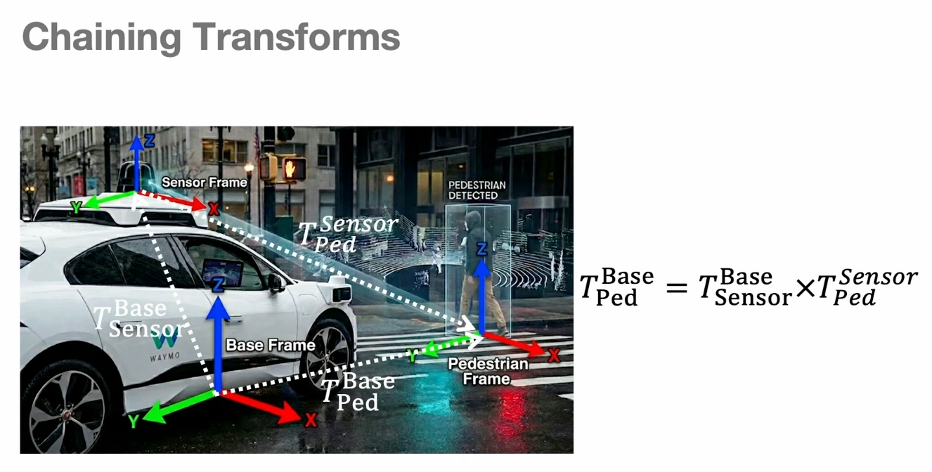
A car might have a base frame at its center, a camera frame on the roof, and a lidar frame somewhere else. If the camera sees a pedestrian, that point is first measured in the camera's local coordinates.
To control the car, we need to transform that point into the base frame. Homogeneous transformation matrices let us chain these frame conversions cleanly.
An articulated robot is a chain of frames
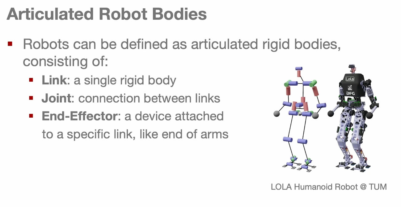
Real robots are usually not one rigid block. A robot arm or humanoid is made of links, joints, and end effectors.
Links are rigid bodies. Joints constrain how links move relative to each other. End effectors are the parts that touch the world, like a gripper or suction cup.
So an articulated robot is basically a chain of coordinate frames connected by joints.
The end effector defines how the robot interacts
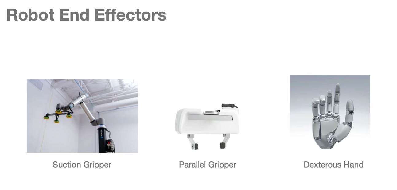
Different end effectors change the action space.
A suction gripper is simple: vacuum on or off. A parallel gripper adds one degree of freedom: open or close to a width. A dexterous hand can have many joints and over 20 degrees of freedom.
The more expressive the hand, the richer the behavior, but the harder the control and learning problem becomes.
Joints are constraints that make motion controllable
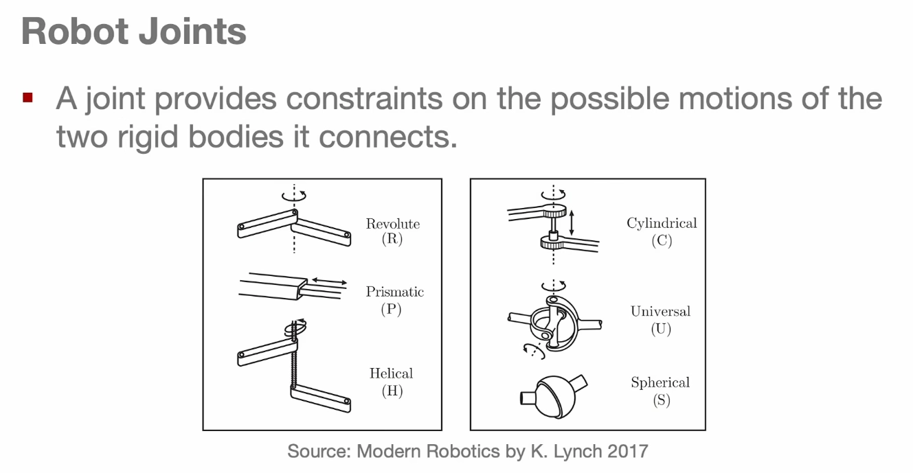
A joint limits the relative motion between two rigid bodies.
The most common joint in robot arms is the revolute joint, which rotates around one axis, like an elbow.
By combining many joints, the robot gains flexibility, but each joint also adds structure to the space the policy must act in.
Degrees of freedom count independent ways to move
Degrees of freedom tell us how many independent parameters are needed to describe the robot's configuration.
A simple planar point has two. A robot arm with many joints may have seven or more. A bimanual system has far more.
A Kutzbach-style way of thinking is to start from possible rigid-body motion and subtract the constraints introduced by joints.
Configuration space is the robot's internal map
Configuration space, or C-space, is the set of all possible robot configurations.
For a robot arm, this is usually the space of joint angles. The geometry can be unintuitive. A two-joint arm with revolute joints forms a torus-like space, because angles wrap around.
This matters for learning: the shortest path between two joint angles may wrap around, not move in a straight Euclidean line.
Workspace is where the robot can physically reach
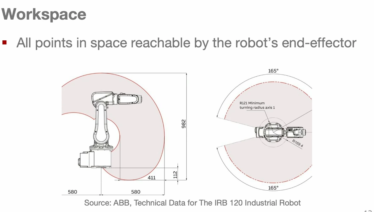
Workspace is the set of physical points the robot can reach in the real world.
The robot perceives many tasks in workspace: a cup on a table, a point on a whiteboard, a block to pick up.
But it executes through configuration space by moving joints. Robot control constantly translates between these two worlds.
Task space is where the goal naturally lives
Task space is the space where the objective is naturally defined.
If the task is cleaning a whiteboard, the task space is the surface of the board. It does not matter whether the robot is a drone, a mobile manipulator, or a humanoid.
The task defines what matters. The robot body defines how that task can actually be executed.
C-space / joint space:
All possible joint angle combinations of the robot.
For 6-DOF arm: [j1, j2, j3, j4, j5, j6]

Task space:
The space where the actual goal is described.
For whiteboard cleaning: [x, y] on the board.
For vacuum cleaning: [x, y] on the floor.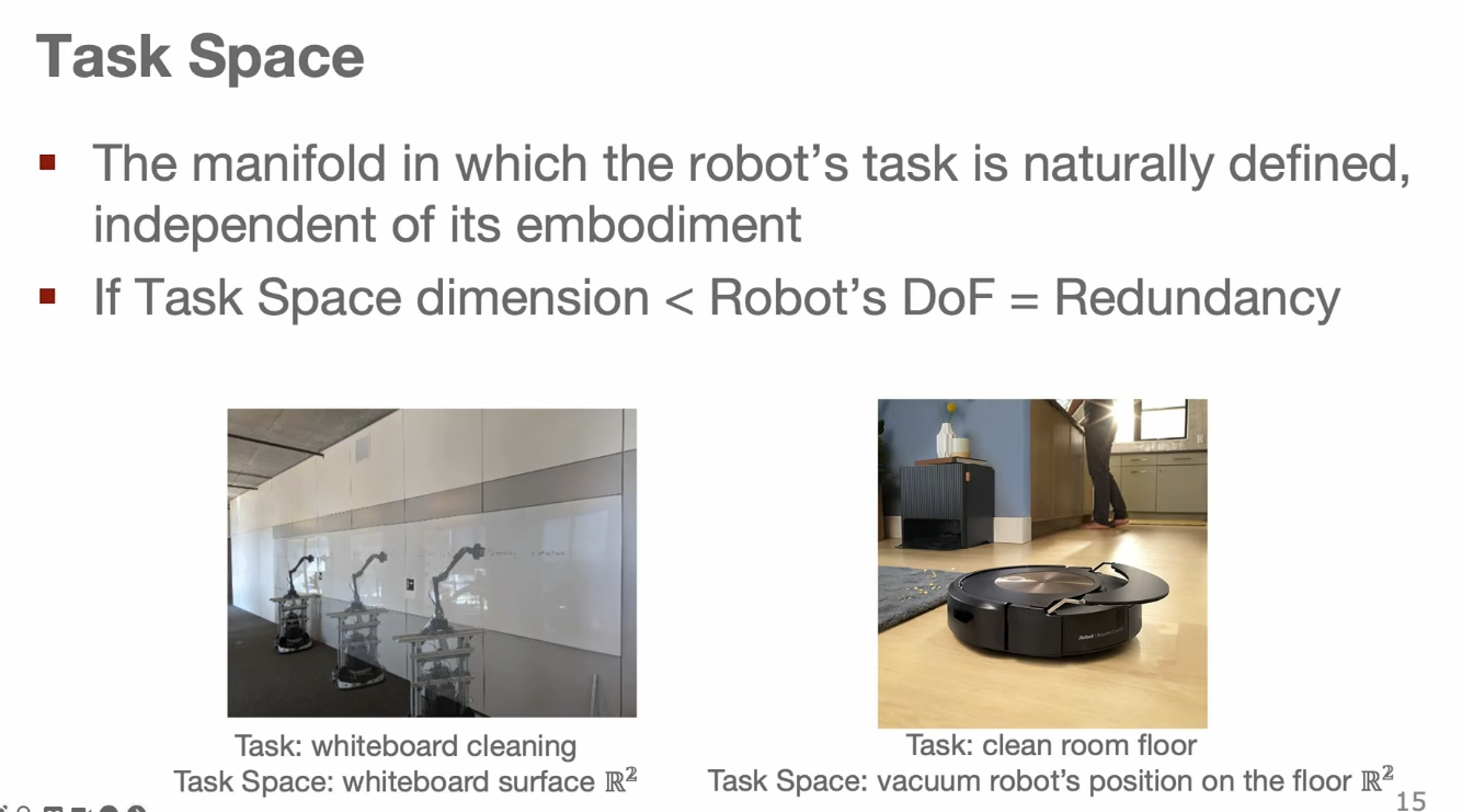
Obstacles become forbidden regions in C-space
An obstacle in workspace maps to a complicated forbidden region in configuration space.
Classical motion planning often worked by explicitly building this C-space, marking forbidden regions, and searching for a path through free space.
That is elegant for low-dimensional robots, but it becomes hard as the number of joints grows.
Learned policies replace hand-built geometry with implicit representations
The old planning style tried to explicitly model all obstacles and geometry.
Modern robot learning often asks the policy to learn these constraints implicitly from data. Instead of hand-building every forbidden region, the model learns that certain observations and actions lead to bad outcomes.
This is the shift from hard-coded geometry to learned representations.
Forward kinematics goes from joints to hand pose
Forward kinematics answers:
given joint angles -> where is the end effector?This direction is deterministic. If you know all the joint values and the robot geometry, there is one resulting end-effector pose.
So forward kinematics is the easy direction of the mapping.
Inverse kinematics goes from desired pose to possible joints
Inverse kinematics asks the harder question:
given desired end-effector pose -> what joint angles should produce it?There can be many valid answers, or no exact analytical solution. Two very different elbow positions can put the hand at the same point.
That is why inverse kinematics is often solved as optimization: minimize pose error while also respecting constraints like joint limits and obstacles.
Redundancy gives the robot room to maneuver
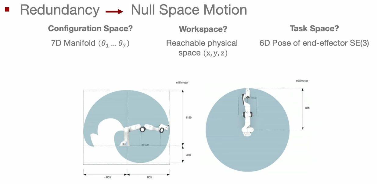
When configuration space has more dimensions than task space, the robot is redundant.
For example, a seven-degree-of-freedom arm may hold a mug steady while still moving its elbow around.
That extra motion is called null-space motion. It can be useful for avoiding obstacles, staying comfortable, or keeping away from joint limits while preserving the task pose.
Why redundancy is useful
If the robot has more DOF than the task requires, it can use the extra DOF to do useful things:
avoid obstacles
avoid joint limits
avoid self-collision
keep the elbow away from the wall
choose a comfortable posture
keep the tool angle stable
move smoothly
reduce energy
So redundancy is not bad. It gives the planner options.
Configuration space vs workspace vs task space
A target pose is not yet a motion
Even after inverse kinematics finds a target joint configuration, the robot cannot teleport there.
It needs a trajectory: a sequence of small waypoints from the current configuration to the target.
So control is not only about where to go. It is also about how to move there smoothly over time.
Linear interpolation is simple but harsh
The simplest trajectory is linear interpolation in joint space.
That gives a straight path between joint configurations, but it causes sharp velocity and acceleration changes at the start and end.
Those jumps stress hardware because the robot is effectively asked to go from still to full motion instantly, then stop instantly.
Quintic trajectories make motion smooth
Industrial controllers often use polynomial trajectories instead of raw linear interpolation.
A quintic trajectory represents each joint motion with a fifth-order polynomial and sets boundary conditions for position, velocity, and acceleration.
The result is a smoother start, smoother stop, and much less violent acceleration behavior.
PID makes the real robot follow the planned path
Even a perfect planned trajectory will not be followed exactly in the real world.
Gravity, friction, inertia, motor limits, and sensor noise all push the robot away from the desired path.
A PID controller closes the loop. Proportional control pulls against current error, integral control compensates persistent bias like gravity, and derivative control damps overshoot.
P = push based on how far you are
I = fix long-term leftover error
D = brake based on how fast you are approaching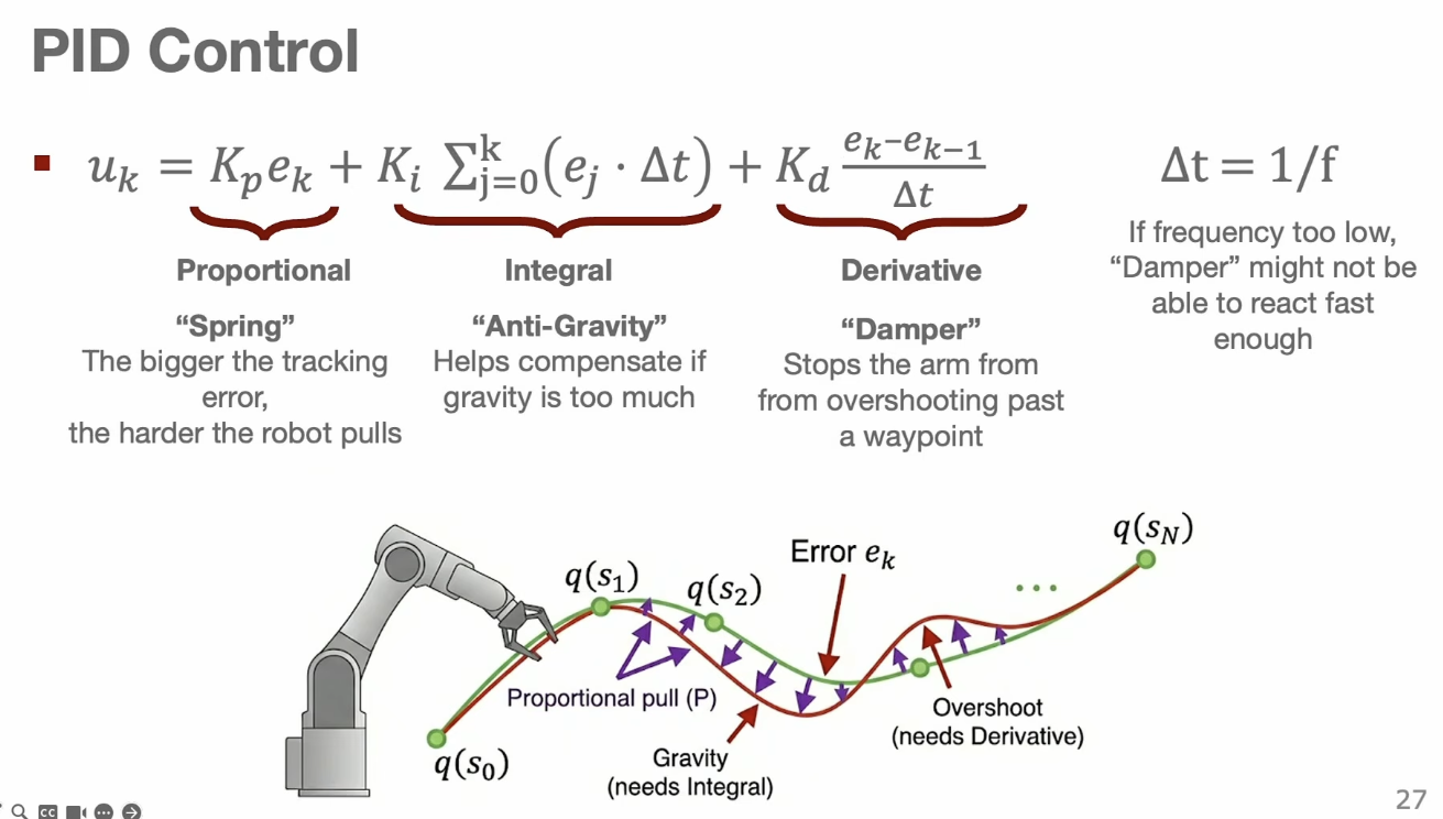
IK → Waypoints → PID mental model
The simple mental model
IK decides where the joints should end up.
Trajectory planning decides how the joints should move over time.
PID makes the real motors follow that planned motion.
The planner gives the “reference path.”
The PID controller fights reality: friction, delay, gravity, motor limits, and small disturbances.
IK:
Where should the joints end up?

Trajectory planning:
How should the joints move there over time?

Collision-aware planning:
How should the joints move there safely?

Time parameterization:
How fast should each part of the motion happen?

PID:
How do we make the real motors follow the planned motion?
Low-level control moves the body; learning chooses the next behavior
Kinematics, interpolation, and PID explain how to execute motion.
But a long-horizon task needs more: the robot must decide which action to take next, under uncertainty, to accomplish a goal.
Bimanual sushi cutting provides a useful example. The low-level controller can follow commands, but the learned policy must decide the sequence of precise actions.
A policy maps observations to action distributions
A neural policy is like a classifier, but its output changes the future world.
An image classifier maps x -> y. A robot policy maps:
observation -> actionMore generally, the policy is a conditional distribution over actions given observations. A stochastic policy assigns probabilities to actions; a deterministic policy puts all probability on one action.
Robot mistakes change the next input
If an image classifier calls a cat a dog, the cat does not change.
If a robot policy steers left into a ditch, the next observation is now from inside or near the ditch.
This is why robot learning is temporally coupled. Actions affect states, states affect observations, and future decisions depend on earlier mistakes.
State is the truth; observation is what the robot sees
The state is the underlying truth: position, velocity, orientation, object locations, and other variables that fully describe the world.
The observation is a partial, noisy view of that state: camera images, proprioception, tactile readings, or lidar.
A snowy night image and a clear day image may give different observations even if the underlying road state is the same.
The Markov property says the current state is enough
The Markov property says that, if you know the true current state, older states do not add extra information for predicting the next state.
In shorthand:
next state depends on current state and actionThe past only matters through what it has already contributed to the current state.
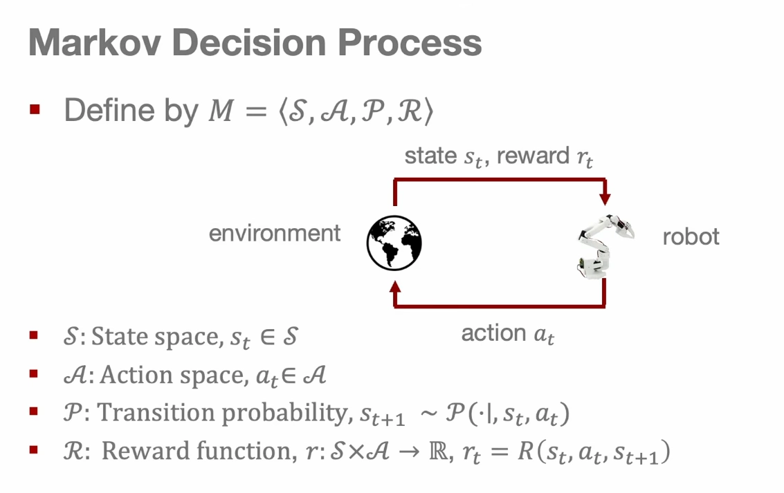
An MDP is the clean math wrapper for robot decision making
A Markov Decision Process packages the robot learning problem into a tuple:
state space, action space, transition dynamics, reward functionThis lets very different systems be described with the same language: a chess player, a self-driving car, a humanoid, or a robot arm.
The hardware changes, but the decision-making structure stays recognizable.
Robotics usually lives in continuous spaces
Some MDPs are discrete. Chess has board squares. A keyboard controller might have a small number of buttons.
Robotics is usually continuous. Joint angles, velocities, gripper widths, and end-effector poses are real-valued.
That means we cannot store a table for every possible state or action. We need function approximators like neural networks.
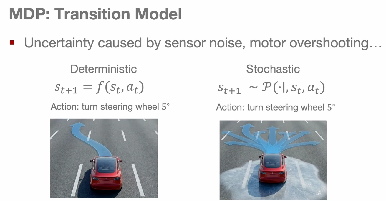
Transitions are stochastic because the world is messy
In an ideal deterministic world, the same state and action always produce the same next state.
Real robots are not like that. Tires slip, motors overshoot, objects shift, sensors are noisy, and contact physics can surprise us.
So MDPs often model transitions as probabilities over next states, not single guaranteed outcomes.
Rewards tell the policy what success means
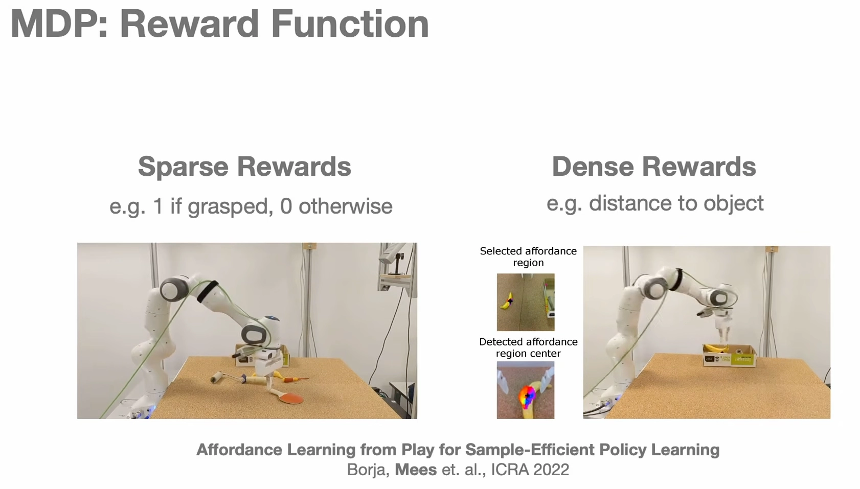
The reward function shapes what the agent tries to do.
A sparse reward might give 1 only when the robot lifts an object and 0 otherwise. A dense reward might also reward reducing the distance between the gripper and the object.
Dense rewards often make learning faster because the policy gets feedback before the final success moment.
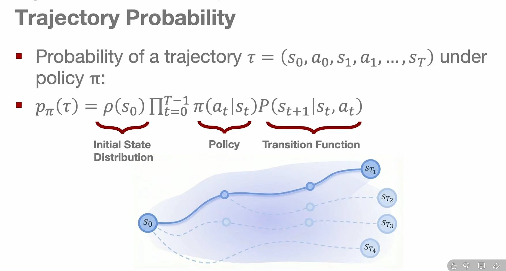
A trajectory is the story generated by policy and physics
A trajectory is a sequence of states and actions:
state_0, action_0, state_1, action_1, ...Its probability comes from three pieces: the initial state distribution, the policy's action choices, and the transition dynamics that determine where the world goes next.
So a trajectory is not just what the robot wanted. It is what the policy and the physics produced together.
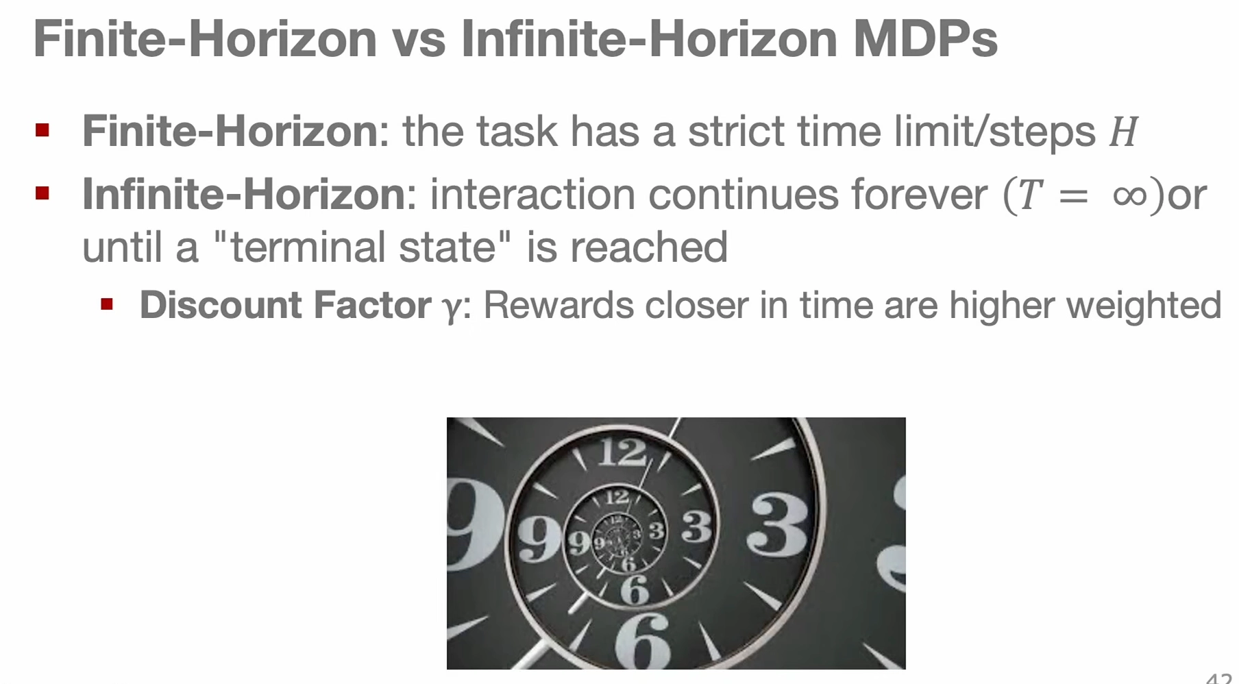
The horizon decides how far into the future the robot cares
A finite-horizon MDP has a fixed end, like five seconds to grab a moving object.
An infinite-horizon MDP can continue indefinitely, like navigation or long-running autonomy.
For long horizons, we usually use a discount factor gamma between 0 and 1, so near-term rewards count more than rewards far in the future.
The learning objective is expected return
The policy should maximize accumulated reward over time.
Because the world is stochastic, we do not optimize one perfect trajectory. We optimize expected return: the average return over all trajectories that could happen when following the policy.
The optimal policy is the strategy that gives the highest expected return under the MDP.
The full bridge is geometry to control to learning
These ideas build a ladder.
First, geometry tells us how to represent robot bodies, frames, joints, and spaces.
Then control tells us how to turn target poses into smooth motion and track that motion on real hardware.
Finally, MDPs tell us how to frame long-horizon decision making so a policy can learn what action to choose next.