Imitation Learning
Notes from Lecture 3 of Robot Learning: From Fundamentals to Foundation Models, taught by Oier Mees.
Imitation learning starts with the idea of copying the expert. Why that simple idea works surprisingly well, and why it quietly breaks once the robot has to live with its own mistakes.
Imitation learning begins by treating expert behavior as the teacher
We assume we have expert trajectories: sequences of states, observations, and actions that successfully complete a task.
The goal is to learn a policy that behaves like the expert. When the robot sees a state or observation, it should output the action the expert would have taken.
For a robot arm, that action might be a joint command, end-effector delta, velocity, or gripper command. For a car, it might be steering.
Behavior cloning is the simplest version
Behavior cloning turns imitation learning into supervised learning.
Each training example is a pair: the observation the expert saw and the action the expert took.
The policy predicts an action, compares it to the expert action, and updates its weights to make the prediction closer next time.
The basic training loop is just regression from state to action
For a deterministic policy, behavior cloning often minimizes a mean squared error between predicted actions and expert actions.
Training looks familiar: sample a batch, run the policy, compute the action loss, backpropagate, and repeat.
This simplicity is why behavior cloning is so widely used in robot learning.
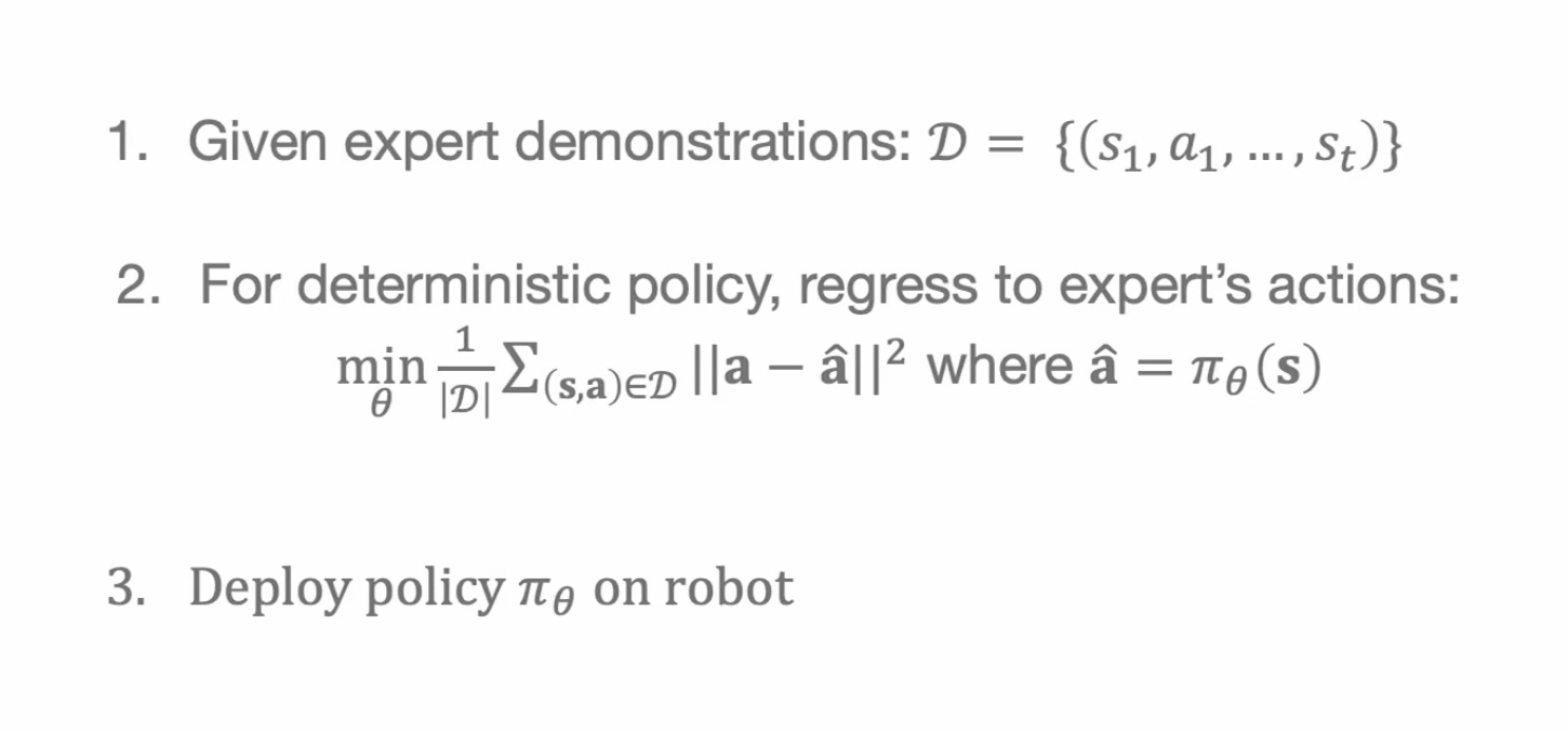
Because it is deterministic:
same state → same action every timeA stochastic policy would instead output a distribution:
same state → maybe action A, maybe action B, with probabilitiesThe first hidden problem is that robot learning is not IID
In ordinary supervised learning, one prediction usually does not change the next input.
If a classifier mislabels one cat image, the next image in the dataset does not change.
In robotics, the policy's action changes the next state. A tiny action error can put the robot somewhere the expert never visited.
Small errors can push the policy off the expert path
Imagine the expert trajectory goes cleanly from state one to state two to state three.
If the learned policy makes a tiny mistake at state one, it may land near state two but not exactly on it.
Now the next observation is already slightly out of distribution, so the next action is more likely to be wrong too.
This is why errors compound
Behavior cloning is trained on states visited by the expert.
At test time, the policy visits states produced by its own actions.
The gap between those two state distributions creates compounding error: one early mistake can create many later mistakes.
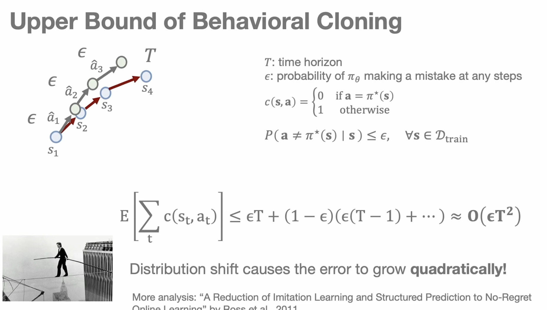
The formal bound says the damage can grow quadratically
If the policy has a small mistake probability on expert states, supervised learning intuition might suggest total error grows roughly linearly with the time horizon.
But after the first mistake, the policy can enter states where its behavior is not controlled by the training data.
That creates a worst-case imitation-learning bound that grows quadratically with the horizon, which is much worse for long tasks.
Behavior cloning still works when the task stays close to the data
The lecture uses end-to-end driving as an early example.
NVIDIA trained a neural network to map camera pixels directly to steering commands, and behavior cloning could produce real driving behavior.
So the point is not that behavior cloning is useless. The point is that it needs help when the deployed policy drifts away from its demonstrations.
Recovery data teaches the policy what to do after mistakes
A self-driving dataset collected only from centered lane driving may not teach the car how to recover from drifting toward the shoulder.
The trick was data augmentation with side cameras.
They added extra “fake” recovery examples:
center camera view → keep going straight
left camera view   → steer right
right camera view  → steer left
So even though the expert was mostly driving correctly, the model also learns:
if I am too far left, correct right
if I am too far right, correct left
The same recovery idea can appear in flying robots
For drones or quadcopters, collecting risky recovery data is hard because humans do not naturally fly through forests.
The lecture describes a similar multi-camera idea: collect visual data from slightly different directions and label it with corrective left, right, or straight commands.
The core idea is the same as driving: create training examples for states the learner may accidentally enter.
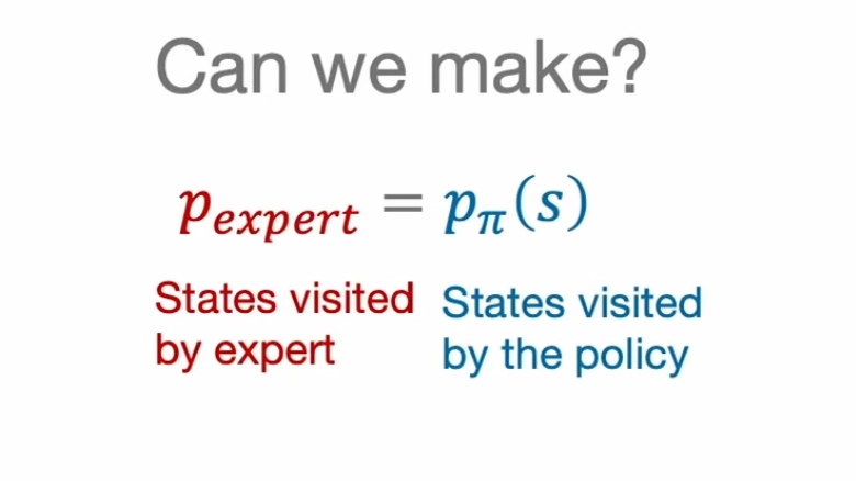
DAgger closes the gap between expert states and policy states
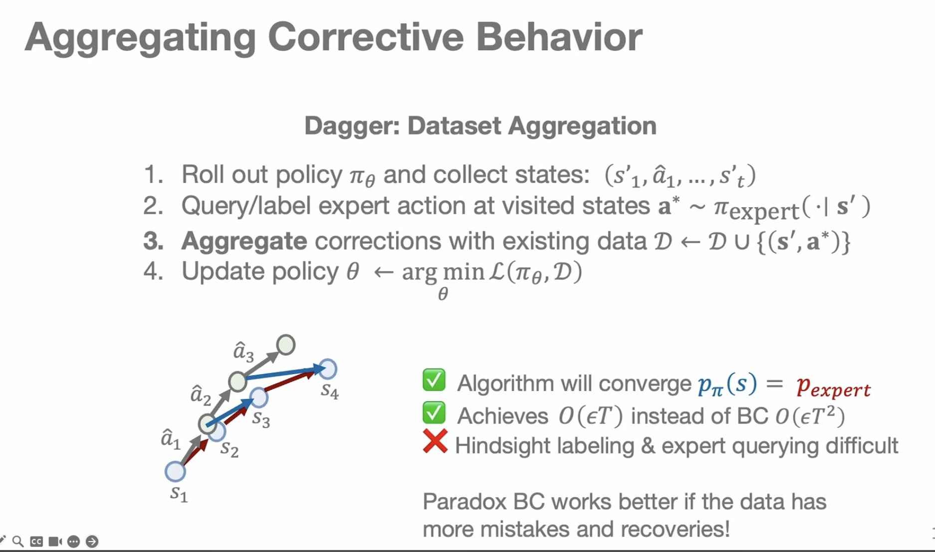
DAgger means dataset aggregation.
We run the learned policy in the environment. When the policy makes mistakes and goes to new states, we ask the expert what the current action should be in those new visited states and add those new label-state pairs back into the dataset.
We update our policy with this new augmented dataset and repeat this process.
You need an expert to label the states your policy visits. That can be expensive, slow, or unsafe on real robots.
The paradox: a dataset with some mistakes and corrections can be better than a dataset with only perfect demos.
DAgger turns deployment mistakes into training data
The reason DAgger helps is that it trains the policy on its own state distribution.
States that were once out of distribution become labeled examples.
Mathematically, this can break the quadratic error growth and recover a much better linear-style bound.
The cost of DAgger is expert labeling
DAgger is powerful, but asking an expert to label every visited state can be expensive.
In robotics, the expert may need to inspect videos, understand the robot state, and provide actions after the fact.
That can be slow, costly, and awkward when the human and robot action spaces do not line up perfectly.
Human-gated DAgger is the driving-instructor version
A more practical variant lets the robot act while a human supervises online.
The human takes over only when the robot starts making a mistake, then provides a corrective partial demonstration.
This is like a driving instructor grabbing the steering wheel only when the student is about to do something unsafe.
Online intervention raises a new question: when should the human step in?
If the human watches constantly, the method can still be expensive.
The robot would ideally know when it is uncertain or close to failure and ask for help before things go wrong.
That turns imitation learning into a question about uncertainty, ambiguity, and when to query a human.
Ambiguous language is one place where asking helps
If a user says fetch the yellow thing and there are multiple yellow objects, the robot should not guess blindly.
It should detect that several objects satisfy the instruction and ask a clarifying question.
It could be a model that identifies candidate objects, generates referring expressions, and asks the human which one they meant.
Clarification is safer than pretending the instruction was obvious
A robot that asks do you mean the middle banana is doing more than being polite.
It is preventing a wrong action before it becomes part of the task trajectory.
This is a practical form of human-in-the-loop imitation: use the human where the model's information is insufficient.
Another failure mode is non-Markovian expert behavior
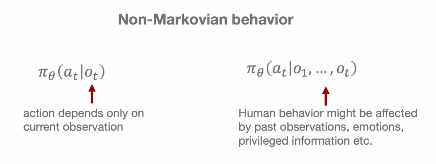
A simple policy assumes the right action depends only on the current observation.
Humans often use history: where an object was moving, what happened a few seconds ago, what they intended, or what they remember from before.
If the same current image can lead to different expert actions depending on history, a memoryless policy is missing information.
Teleoperation can also give the human privileged information
The human demonstrator may see more than the robot policy sees.
During teleoperation, the operator can look around, use extra context, or infer hidden state that is not present in the robot's camera observation.
Then the dataset contains actions that make sense to the human, but the policy cannot infer why from its own inputs.
Adding history can help, but it is not free
A natural fix is to feed the policy multiple past frames or observations.
Then an LSTM, RNN, transformer, or other sequence model can condition actions on history.
This can resolve some non-Markov behavior, such as tracking a cyclist's motion before deciding how to drive.
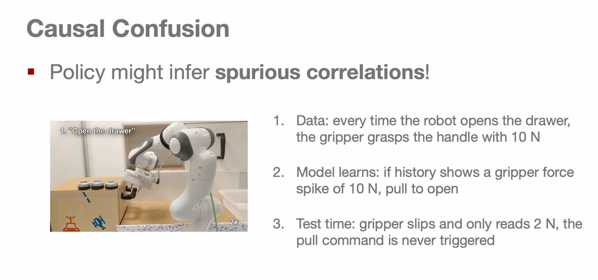
History can create causal confusion
High-capacity models look for the easiest way to reduce loss, not necessarily the right causal reason.
If a force sensor spike often appears before a drawer pull, the model may learn to wait for that spike instead of understanding that the gripper is holding the handle.
When the real sensor value shifts, the learned shortcut breaks.
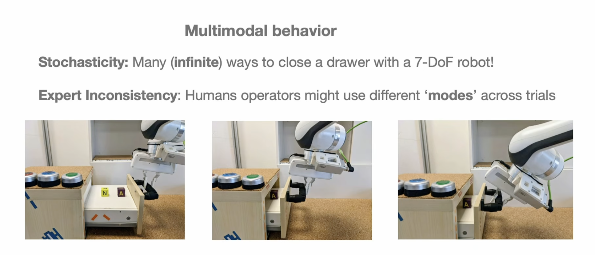
The biggest modeling problem is multimodal expert behavior
In robotics, multimodal data usually means: for the same or similar situation, there are multiple valid behaviors or actions.
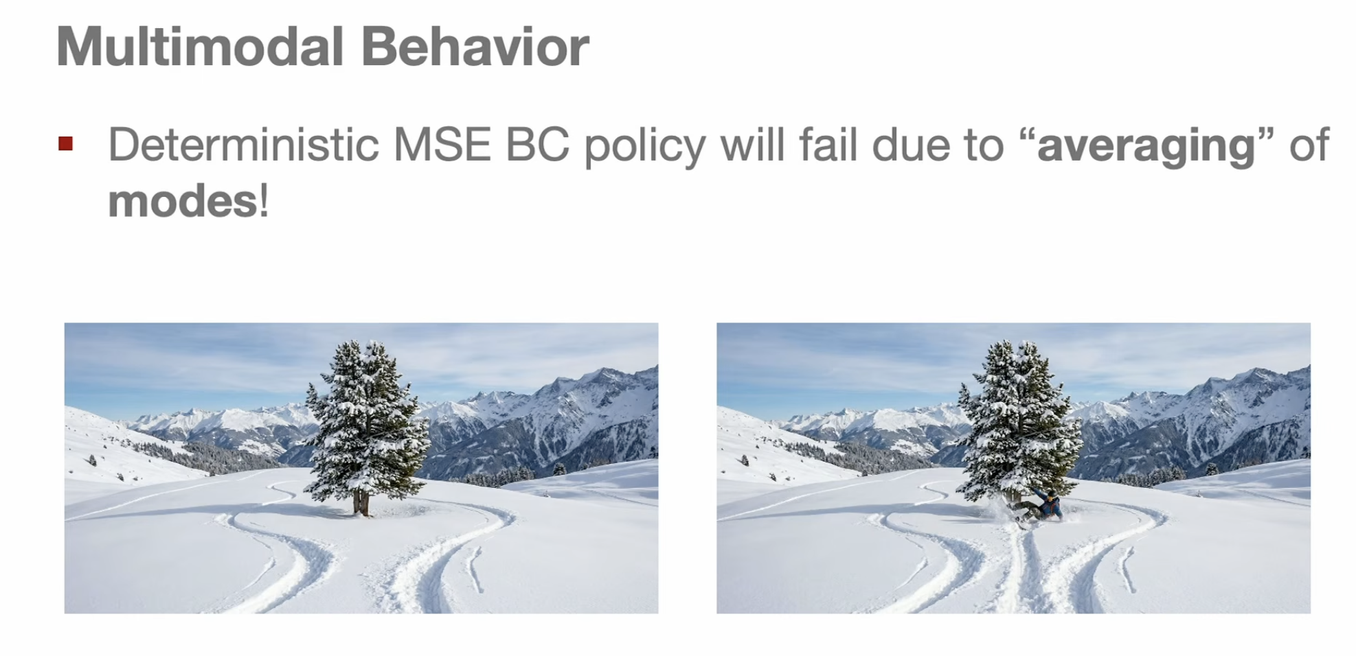
Mean squared error averages modes into bad actions
If one expert goes left around an obstacle and another goes right, the average action may go straight into the obstacle.
This is the classic problem with using a single Gaussian-style regression target for multimodal behavior.
The average of good actions is not necessarily a good action.
There are two data points: one going on from the left side of the tree and one going from the right side of the tree. It will average out and it will hit the tree.
Mixture models are the first multimodal fix
A mixture of Gaussians can represent several peaks in the action distribution.
Each component can capture a different valid behavior mode.
The limitation is that you often need to choose how many modes to represent, and high-dimensional robot actions can make this difficult.
The average is inconsistent with the expert data. A single Gaussian action model assumes there is one main best action peak, so it may average the two actions. But the middle action might be bad, like driving straight into the obstacle.
Single Gaussian: one blob of possible actions
Mixture of Gaussians: many blobs of possible actions
Discretization turns action prediction into classification
Another option is to divide continuous actions into bins and predict action tokens.
This can represent multiple likely bins instead of collapsing everything into one average.
The difficulty is dimensionality: naive discretization grows very quickly as the number of action dimensions increases.
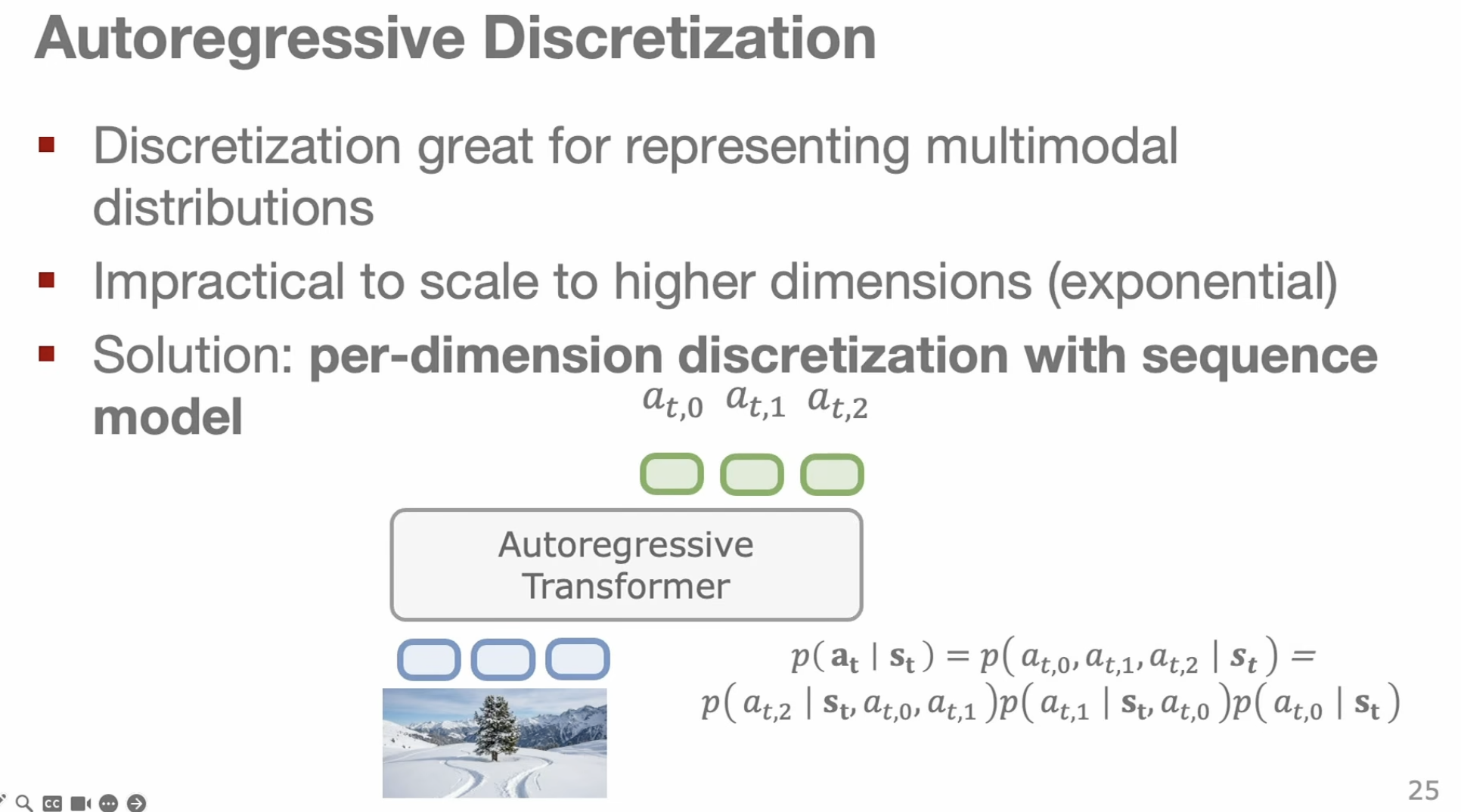
Autoregressive action tokens reduce the dimensionality problem
Instead of predicting one giant discretized action grid, the model predicts action dimensions one by one.
This makes the number of predictions scale more gently with the number of dimensions.
The tradeoff is sequential computation: the model may need to generate many action tokens before it has a full action vector.
Autoregressive discretization is great for representing multimodal distributions, so it can represent multiple peaks, unlike a single Gaussian. But if the action has many dimensions, discretizing the whole action at once becomes huge. The solution is per-dimension discretization with an autoregressive model.
Another way to address multi-modality is generative modeling
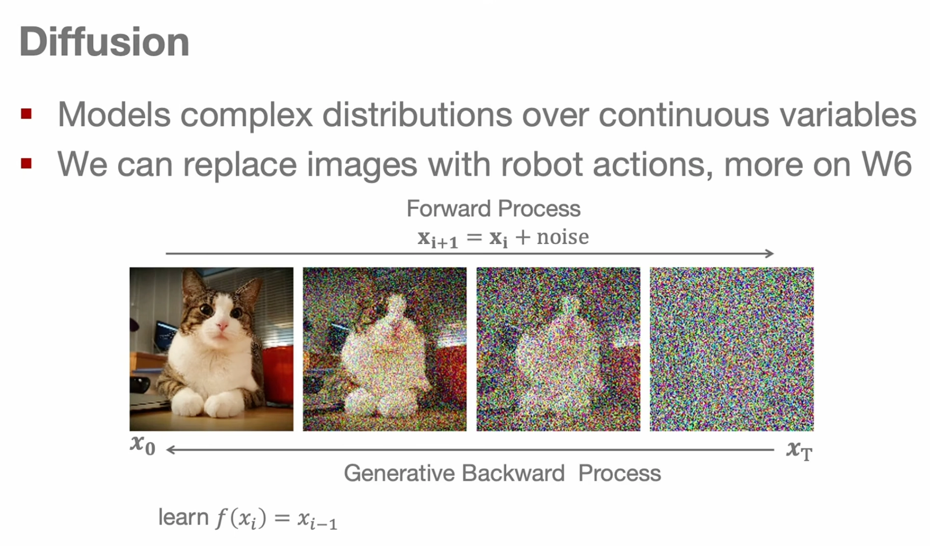
Diffusion gives another way to model multimodal action distributions.
During training, clean action trajectories are corrupted with noise, and a network learns to denoise them step by step.
At test time, the policy starts from noise and iteratively produces a plausible action sequence conditioned on the observation.
Latent variable policies use a hidden plan to choose a mode
A latent variable model gives the policy an extra sampled variable, often called z.
That latent acts like a mode or style selector: approach from the left, approach from the right, grasp high, grasp low, and so on.
The policy can then represent many possible successful behaviors without averaging them into one blurry action.
The latent plan is not the same as the task
The task specification tells the robot what goal to achieve, such as open the drawer.
The latent plan tells the robot which style or route to use within that task.
Many latent plans can solve the same task, because the world is continuous and there are many valid ways to reach the goal.
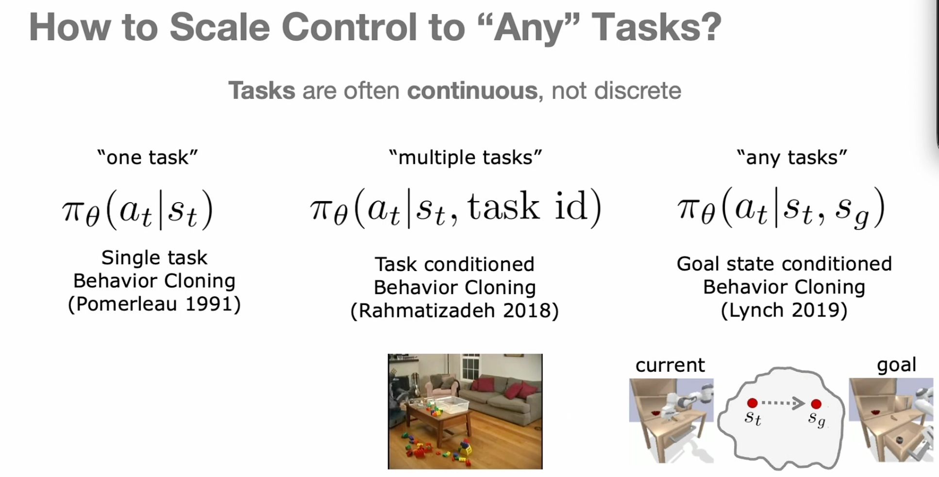
Goal reaching is broader than discrete task IDs
Real-world tasks do not always have clean boundaries.
Moving a sliding door halfway might be enough for one purpose and not enough for another.
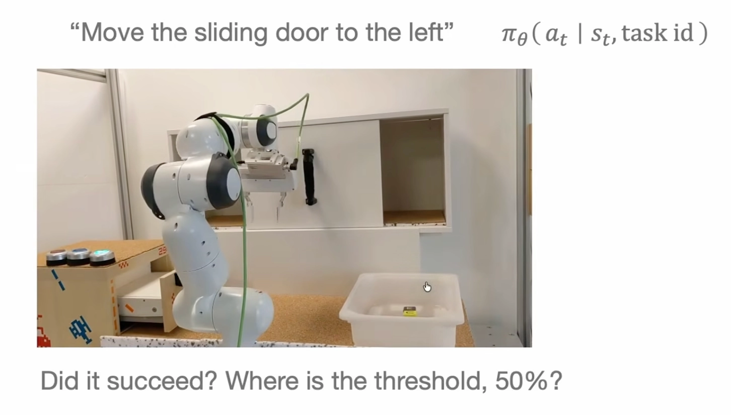
Goal-conditioned learning reframes the problem as reaching a desired goal state from a current state, which better matches the continuous nature of robot behavior.
Play data removes the need to predefine every task
In play data, a human teleoperates the robot freely and explores the environment without strict task labels or resets.
This produces unstructured, multimodal data with many transitions between many states.
It is closer to how children learn: curiosity-driven interaction creates a broad set of skills before anyone names each task.
Play-LMP learns latent plans from random windows of play
The model samples a short window from play data.
The first frame becomes the current state, the last frame becomes the goal, and the actions in between become the behavior to imitate.
A posterior encoder reads the actual sequence and infers the latent plan; a prior learns to propose likely plans from the current state and goal.
At test time, the posterior disappears
During training, the posterior can see the demonstrated future behavior, so it can infer which latent plan was used.
At test time, the robot does not have the future trajectory.
It uses the learned prior or plan sampler to choose a plausible latent plan, then the decoder turns that plan into actions.
Learning policies from play data in more detail
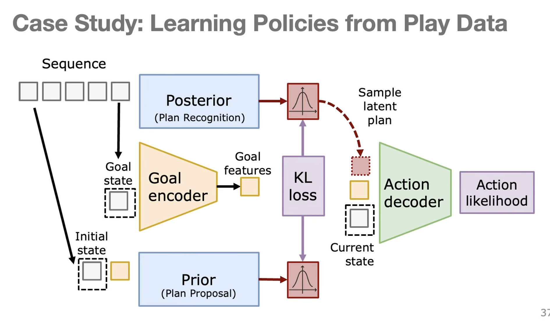
This shows how to learn a robot policy from play data without manually labeling tasks.
Core idea:
Long play sequence
→ choose an initial state and a goal state
→ learn what actions move from current state toward that goal
The model has a hidden variable called a latent plan. Think of latent plan as:
“what style/strategy should I use to reach the goal?”Example:
Goal: object inside bowl

Plan 1: grasp object, lift, place
Plan 2: push object into bowl
Plan 3: slide object closer, then grasp
What each block does
Goal encoder: looks at the goal state and converts it into goal features.
goal image/state → compact goal representationPosterior / Plan recognition: during training, it sees the full sequence, so it can infer:
“What plan was probably used in this demo?”Prior / Plan proposal: at test time, you do not have the future sequence. You only know the current state and goal. So the prior learns to propose a likely plan from those.
current state + goal → possible latent planKL loss: this makes the prior's guessed plans match the posterior's inferred plans.
prior should learn to guess the kind of plan the full sequence would implyAction decoder takes current state, goal, and sampled latent plan, then predicts the action.
The latent plan lets the robot represent many possible ways to reach the same goal.
Without latent plans:
same goal → average of many behaviors → bad action

With latent plans:
same goal + plan A → push
same goal + plan B → grasp
same goal + plan C → slide
So the model can learn rich, multimodal behavior from messy play data.
The VAE objective has two jobs
The reconstruction term asks whether the latent plan explains the demonstrated action sequence.
The regularization term asks whether the posterior stays close to the prior, so the test-time sampler can produce useful plans.
This is the core reason CVAE-style policies can learn from messy multimodal play data.
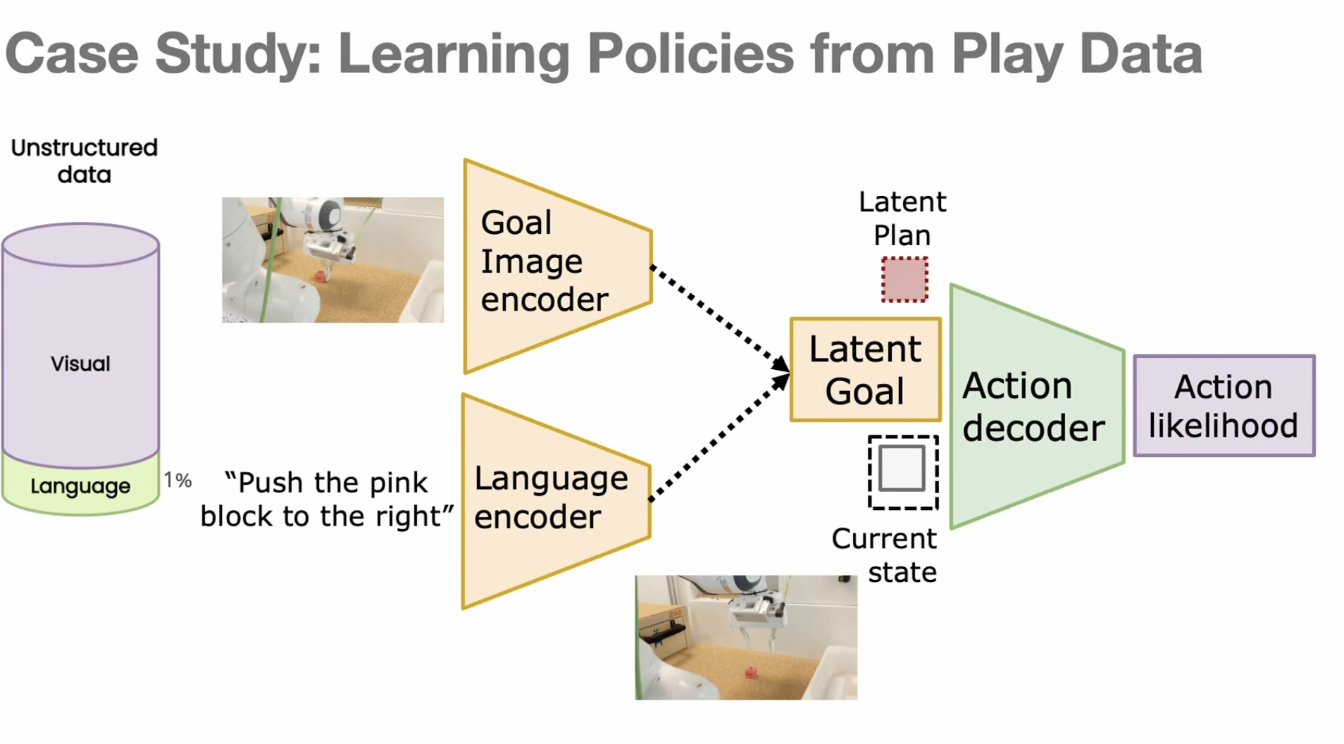
Language goals can piggyback on visual goal learning
The lecture notes that we can swap visual goals with embeddings of natural language goals.
That lets the robot learn mostly from unlabeled play data while using a small amount of language annotation to connect words to behaviors.
This reduces the burden of labeling every demonstration with natural language.
The final toolkit is not one trick, but several layers
Behavior cloning gives the basic supervised imitation recipe.
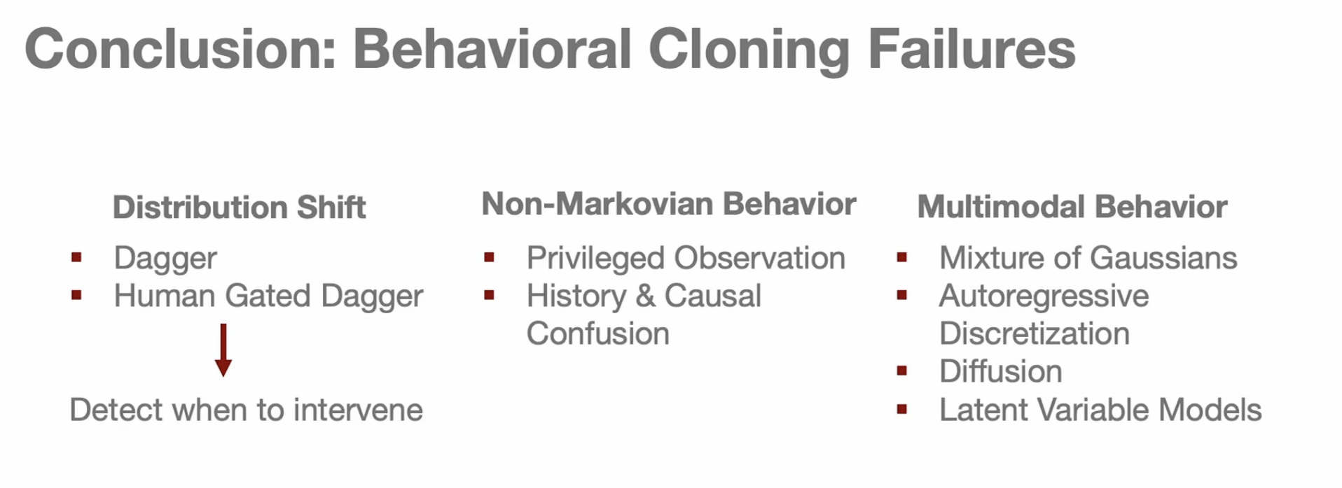
DAgger and online intervention address distribution shift. History addresses partial observability. Mixtures, discretization, diffusion, and latent variables address multimodal actions.
Goal reaching and play data widen the scope from fixed tasks to the continuum of behaviors available in an environment.
The math behind goal-conditioned latent variable models
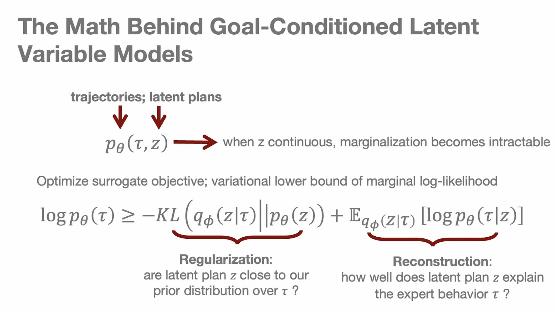
But if z is continuous, there are infinitely many possible plans.
z could be 0.01, 0.011, 0.0111, ...So computing the exact probability by checking all z becomes too hard. That is intractable marginalization.
Since the exact objective is too hard to compute, we optimize a replacement objective. That replacement is called a surrogate objective.
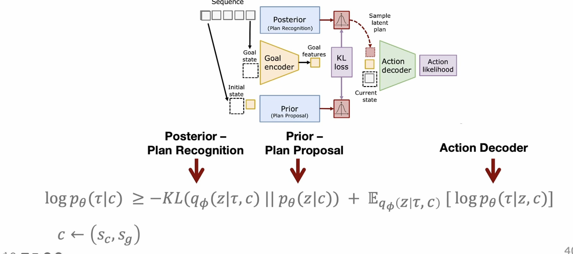
c = (s_c, s_g)means the condition: current or start state plus goal state.
The model has three main parts:
1. Posterior / plan recognition
qϕ(z | τ, c)This sees the full trajectory τ during training and infers what latent plan z explains this behavior. It is the training-time network that finds the plan from what actually happened.
2. Prior / plan proposal
pθ(z | c)This only sees the current state and goal. It learns to propose a likely latent plan without seeing the future trajectory. This is what you use at test time.
3. Action decoder
pθ(τ | z, c)Given condition c and latent plan z, it tries to reproduce or predict the trajectory and actions.
reconstruction term:
Does z explain the actual trajectory?

KL term:
Make the posterior's inferred z close to the prior's proposed z.
Training:
trajectory + goal → posterior finds useful z
decoder uses z to explain actions
KL teaches prior to propose similar z
Testing:
current state + goal → prior samples z
decoder turns z into actionsThe key intuition: posterior learns plans from full examples, prior learns to guess those plans when only given the current state and goal.
The lecture's core message
Imitation learning is powerful because it turns robot policy learning into a familiar supervised problem.
It is fragile because robots act into the world, shift their own inputs, inherit human inconsistencies, and face many valid ways to solve the same task.
Modern imitation learning is the art of keeping the simplicity of copying experts while adding the machinery needed for distribution shift, memory, multimodality, and open-ended goals.