Generative Modeling
Notes from Lecture 6 of Robot Learning: From Fundamentals to Foundation Models, taught by Oier Mees.
Robot behavior is rarely a single correct action. Generative modeling gives us tools for representing full distributions of possible behaviors instead of forcing the policy to average them into one brittle action.
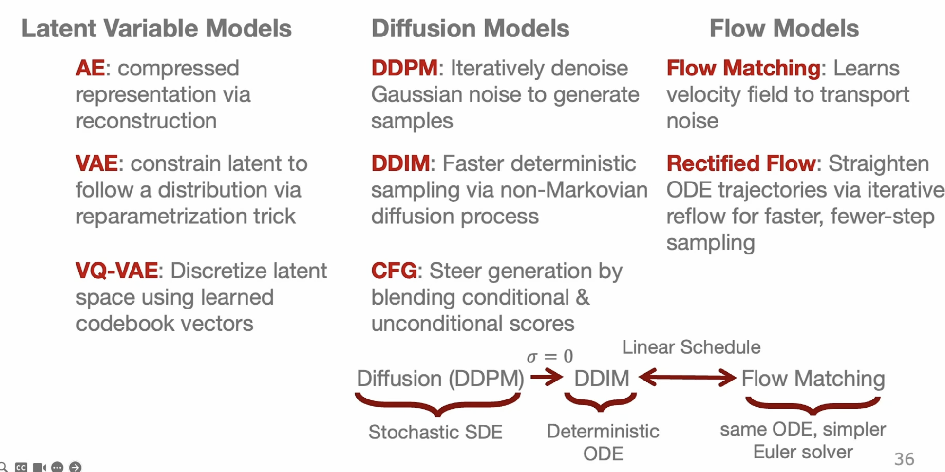
Generative modeling matters because robot actions are not just a function
In robotics, the mapping from observation to action is often not one clean deterministic function.
It is closer to a distribution.
same observation -> many valid actionsThere are two main reasons.
First, the robot body itself creates many possibilities. A high degree-of-freedom arm may reach the same goal in many different ways.
Second, human demonstrations are inconsistent. One expert might grasp from the side, another from the top. Even the same expert may move faster one day and slower another day.
So the policy should not only answer:
What is the one action?It should answer:
What distribution of actions makes sense here?MSE behavior cloning can average good actions into a bad one
If we train a deterministic policy with mean squared error, the model is pushed toward the average of the demonstrations.
That is fine if the data has one mode.
But if there are multiple valid behaviors, averaging can produce something invalid.
expert path 1: go left around obstacle
expert path 2: go right around obstacle
MSE average: go straight into obstacle
This is the classic multimodality problem.
The average of two good actions is not always a good action.
Generative models are useful because they try to represent the full distribution, not just its mean.
A generative model maps simple noise into complex data
At a high level, a generative model learns a transformation.
simple distribution -> complex data distributionThe simple distribution is usually something tractable, like a standard Gaussian.
z ~ N(0, I)The complex distribution might be:
images
videos
robot action trajectories
latent plans
So the goal is not just compression. The goal is to learn how to sample new things that look like the data distribution.
For robot learning, this means sampling plausible behaviors or action sequences.
Autoencoders begin with compression
A basic autoencoder has two parts.
encoder: x -> z
decoder: z -> reconstructed x
The encoder compresses the input into a smaller latent representation. The decoder tries to reconstruct the original input.
The bottleneck forces the model to preserve the important structure in the data.
input data -> compact code -> reconstructed dataThis is self-supervised because we do not need labels. The input itself becomes the reconstruction target.
But a plain autoencoder is not yet a strong generative model.
Plain autoencoders compress, but their latent space has no useful sampling structure
A deterministic autoencoder maps each input to one point in latent space.
That creates a few problems.
one input -> one latent pointThe latent space can be messy. Clusters can appear anywhere, and nothing forces nearby latent points to decode into meaningful nearby outputs.
The only real constraint is the bottleneck size.
Most importantly, sampling is not well-defined. If we randomly pick a latent point, the decoder may have never seen anything like it during training.
So the model can reconstruct, but it does not automatically know how to generate safely.
VAEs turn the latent code into a distribution
A variational autoencoder changes the encoder output.
Instead of producing one latent point, the encoder predicts a distribution.
encoder(x) -> mean and variance
sample z from that Gaussian
decoder(z) -> reconstructed x
Now the latent representation is stochastic.
This matters because at test time we can sample from the prior:
z ~ N(0, I)
decoder(z) -> new sample
So the VAE becomes a real generative model: it can create new outputs by sampling latent variables.
VAE in robotics test and training
Think of a VAE-style robot policy as behavior cloning with a learned action generator.
During training, the model sees:
current camera images
current robot state
expert action chunk from t to t+H
The encoder compresses the expert action chunk into a latent plan z.
expert future actions -> encoder -> mean, variance -> zThe decoder then tries to reconstruct the same action chunk from:
current observation + robot state + zSo z can represent the style or plan of the movement:
approach from left
grasp slowly
use this wrist angle
lift after closing
At test time, the robot does not have expert future actions. It only has the current images and robot state. So it samples a latent plan or uses a default one:
z ~ N(0, I)Then the decoder predicts the next action chunk.
camera images + robot state + z -> next H actionsThe robot executes the first action or first few actions, observes again, and repeats. This is receding horizon control.
Main idea:
training: learn how expert action chunks map to latent plans
test time: sample a latent plan and generate a plausible action chunk
The VAE part lets the same visual situation produce different valid action styles instead of forcing the policy to average them.
The VAE objective balances reconstruction and latent structure
A VAE wants two things at the same time.
First, it should reconstruct the input well.
sample z from encoder distribution
decoder(z) should recover x
Second, the encoder's distribution should stay close to the prior.
q(z | x) should not drift too far from N(0, I)This gives the ELBO objective.
reconstruction term
+
KL regularization term
The reconstruction term makes outputs accurate. The KL term makes latent space sampleable.
Without the KL term, the latent space can become an unstructured storage system again.
The reparameterization trick moves randomness to the side
Sampling creates a gradient problem.
If z is sampled from a distribution predicted by the encoder, it is hard to backpropagate through the sampling operation directly.
The reparameterization trick rewrites the sample as:
z = mu + sigma * epsilon
where epsilon ~ N(0, I)
Now the randomness is in epsilon, which does not depend on the encoder parameters.
The encoder only produces mu and sigma, which are normal differentiable outputs.
So the gradient can flow through:
loss -> decoder -> z -> mu, sigma -> encoderThis is why VAEs can be trained efficiently with gradient descent.
REINFORCE could handle sampling, but it is too noisy here
The lecture connects this back to policy gradients.
One way to handle gradients through sampling is the score-function estimator, the same idea behind REINFORCE.
grad expectation -> expectation of grad log probability * reward/lossBut this has high variance because the gradient does not see how the sampled z itself changes with encoder parameters.
The optimizer only learns whether a sample was good or bad.
The reparameterization trick is better here because it gives a pathwise gradient.
how should mu and sigma move to make z better?That signal is much more direct.
VAEs can still fail by ignoring the latent or hallucinating between modes
VAEs are powerful, but two failure modes matter for robotics.
First: posterior collapse.
If the decoder is too strong, it can learn to reconstruct without using z much.
powerful decoder -> ignores latent code -> weak generative structureSecond: prior mismatch.
Suppose the data has two modes:
left behavior
right behavior
The VAE prior may let us sample a latent point in the middle. But the decoder may never have seen training examples from that middle region.
In images, this may create a strange blurry sample. In robotics, it could create an unsafe action.
VQ-VAE replaces continuous latents with a discrete codebook
A vector-quantized VAE uses a learned dictionary of latent codes.
codebook = k learned vectors
encoder output -> nearest codebook vector
decoder receives that discrete code
So instead of passing a continuous latent vector to the decoder, we snap it to the nearest learned code.
This forces the model to choose from a finite vocabulary.
continuous signal -> discrete tokenThat helps avoid some of the fuzzy middle regions that continuous VAEs can create.
It also makes the representation more transformer-friendly, because the data can be treated as sequences of tokens.
The straight-through estimator pretends quantization was differentiable
The nearest-neighbor lookup in VQ-VAE is not differentiable.
encoder output -> argmin nearest codeSmall changes to the encoder output often do not change the selected code at all, so the true gradient is zero almost everywhere.
The straight-through estimator uses a practical hack.
forward pass: use quantized code
backward pass: copy gradient through as if quantization did not happen
This is not the exact mathematical gradient, but it works as a useful proxy.
The intuition: if the encoder output and selected code live close together in the same embedding space, then the decoder gradient for the selected code is a reasonable signal for how the encoder output should move.
VQ-VAE training has reconstruction, codebook, and commitment losses
The VQ-VAE loss has three pieces.
First is reconstruction.
decoded quantized code should reconstruct the inputSecond is codebook learning.
move codebook vectors toward encoder outputsThird is commitment.
make encoder outputs stay close to selected codebook vectorsThe commitment loss matters because the straight-through gradient assumes the encoder output and quantized code are close.
If they drift far apart, the copied gradient becomes a bad proxy.
To generate with VQ-VAE, we train a prior over code sequences
A trained VQ-VAE gives us an encoder, a codebook, and a decoder.
But to generate new samples, we need to know which codes to pick.
So VQ-VAE often has a second training stage.
1. encode dataset into code indices
2. train a prior model over those code sequences
3. sample new code indices from the prior
4. decode codes into data
The prior can be an autoregressive transformer.
This turns continuous data into a token modeling problem.
image/video/action trajectory -> sequence of discrete codesVQ-VAE is useful because it tokenizes robot learning problems
VQ-VAEs are useful beyond image compression.
They can tokenize:
images
videos
latent plans
actions
motion between frames
In robot learning, this is powerful because many modern models are transformer-based.
Transformers like tokens. VQ-VAE gives them tokens for continuous signals.
Examples from the lecture include tokenizing visual data, learning latent action codes from videos, quantizing plans from play data, and discretizing continuous robot actions for vision-language-action models.
The big idea is:
continuous robot experience -> discrete symbols -> sequence model can reason over itDiffusion models avoid a latent bottleneck and learn to denoise
VQ-VAE still has limitations. For example, reconstruction losses like MSE can still create mean-seeking outputs.
Diffusion models take a different route.
Instead of compressing into a bottleneck, they model the full continuous data distribution by learning a denoising process.
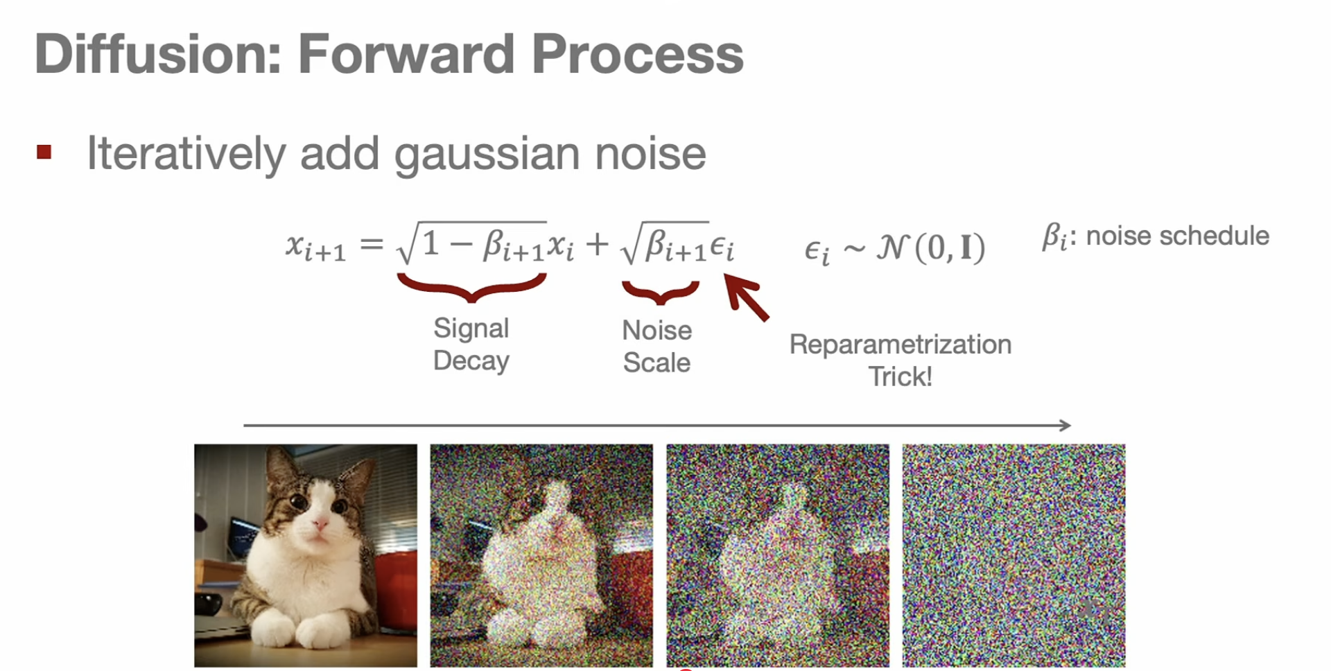
The forward process destroys data:
clean sample -> add noise -> more noise -> almost pure noiseThe reverse process learns to undo that destruction:
noise -> denoise step -> denoise step -> clean sampleSo generation becomes iterative refinement rather than one-shot prediction.
Diffusion is easier because each step makes a small correction
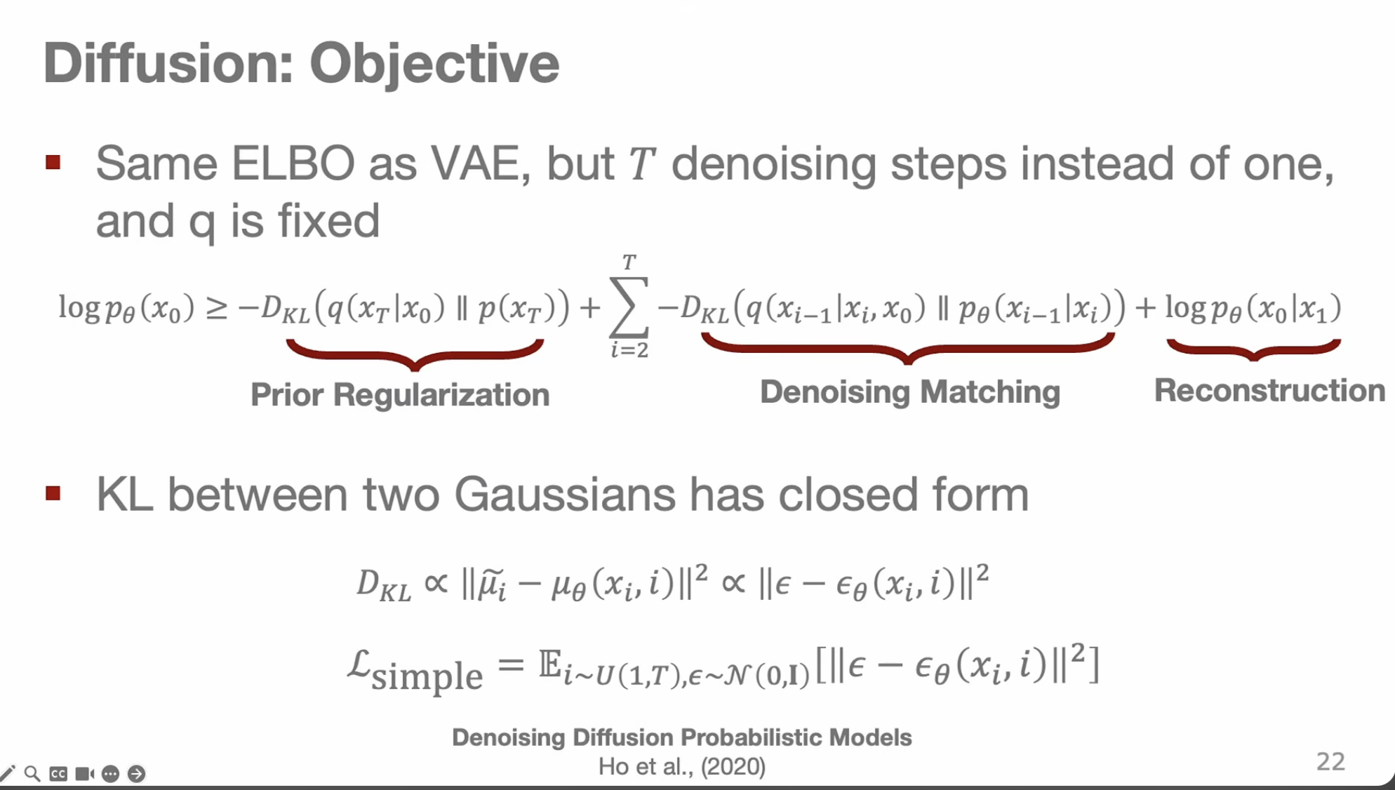
Predicting a full image or full action trajectory in one shot is hard.
Diffusion asks a smaller question at each step:
Given this noisy sample and timestep,
what noise was added?
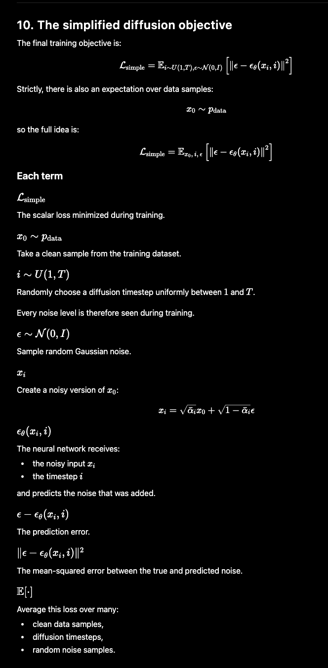
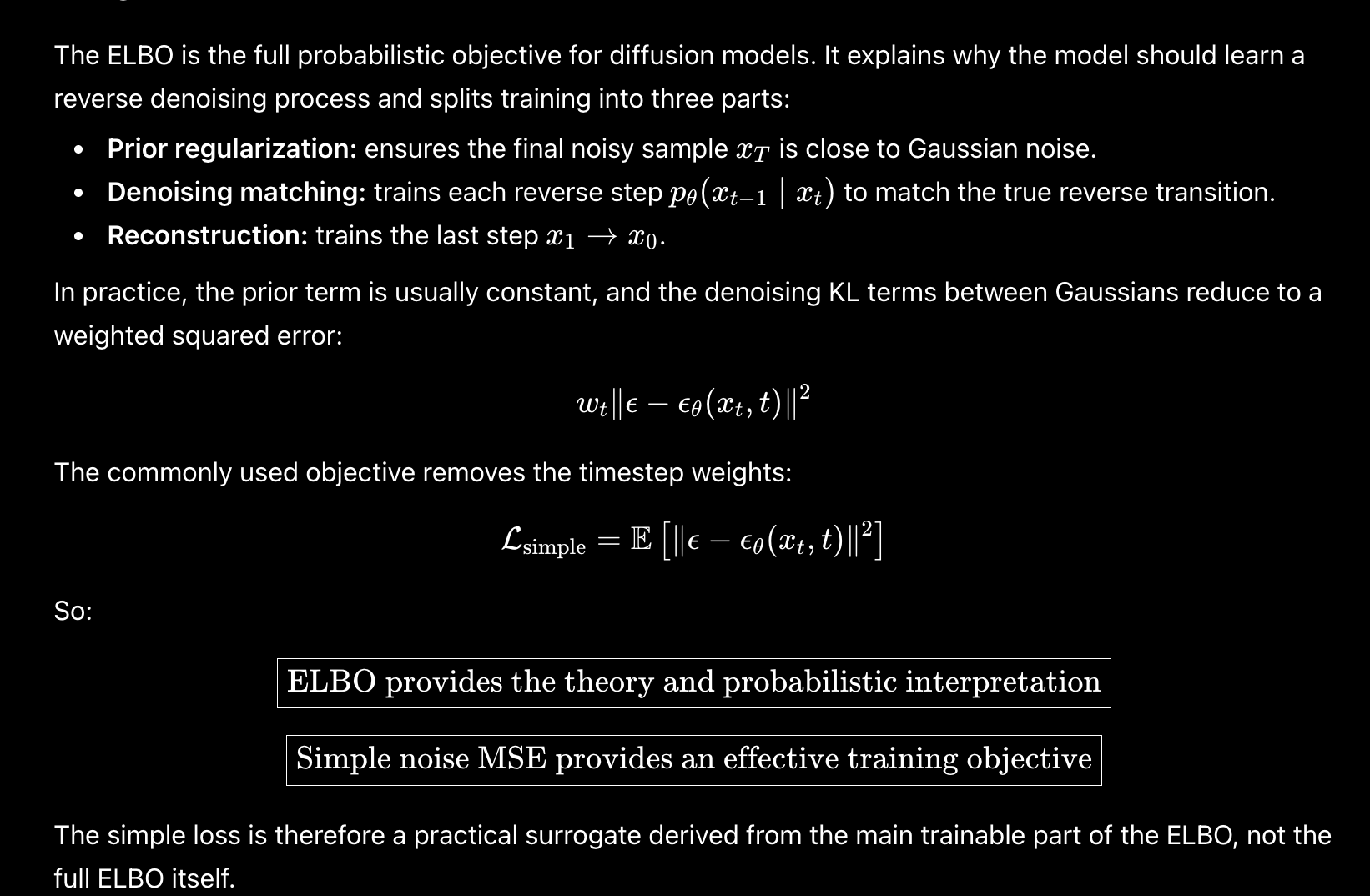
The model learns to predict the noise, not directly the clean sample.
That is useful because the noise is known during training.
true noise epsilon
predicted noise epsilon_theta
loss = MSE(epsilon, epsilon_theta)
Each denoising step is a local correction. Many local corrections together produce a high-quality sample.
The forward process can jump directly to any noise level
Naively, to get x_t, we might add noise step by step from x_0.
x0 -> x1 -> x2 -> ... -> xtThat would be expensive during training.
Diffusion has a closed-form shortcut: because sums of Gaussians are Gaussian, all the intermediate noise can be collapsed into one noise sample.
So we can sample any timestep directly:
x0 + one scaled Gaussian noise sample -> xtThis makes training efficient because we can randomly choose a timestep and train the denoiser there without simulating all earlier steps.
Diffusion: Objective
DDPM sampling adds noise back to preserve diversity
In DDPM sampling, we start from Gaussian noise and denoise step by step.
At each step, the model predicts how to move toward a cleaner sample.
But DDPM also adds some noise back during sampling.
That sounds strange at first:
denoise
then add noise again
The reason is diversity. If the reverse process were purely deterministic, samples could collapse toward the same mean.
The added stochasticity helps the model explore the full distribution instead of producing one average-looking output.
DDIM makes diffusion sampling faster by becoming deterministic
DDPM can require many denoising steps, often hundreds or thousands.
That is slow for robotics, where actions may need to be produced quickly.
DDIM decouples training timesteps from inference timesteps.
train with many noise levels
sample with fewer denoising steps
DDIM removes the extra stochastic noise term during sampling, making the trajectory deterministic.
This allows bigger jumps through time.
T=100 -> T=80 -> T=60 -> ... -> clean sampleFor robot policies, fewer sampling steps can be the difference between elegant theory and usable control.
Conditioning tells the generative model what we want
Unconditional generation is usually not enough.
For images, we want to condition on a prompt. For robots, we want to condition on observations and tasks.
condition c = camera image, robot state, language command, goal imageThe simple approach is to give the condition to the denoising network.
noisy sample + timestep + condition -> predicted noiseBut the model may learn to ignore the condition if unconditional denoising is easier.
So conditioning needs some extra care.
Classifier-free guidance teaches both conditional and unconditional denoising
Classifier-free guidance trains one model in two modes.
During training, the condition is randomly dropped sometimes.
with condition -> conditional denoising
without condition -> unconditional denoising
At inference time, we compare the two predictions.
conditional prediction - unconditional predictionThat difference tells us the direction the condition wants to push the sample.
The guidance scale controls how strongly we follow it.
higher guidance -> more condition-following
lower guidance  -> more diversity
This same idea carries over from image generation to robot action generation.
Diffusion Policy treats actions like the thing being generated
Diffusion Policy applies diffusion to robot control.
The key move is simple:
replace pixels with robot action sequencesInstead of denoising an image, the model denoises a chunk of future actions.
noisy action sequence + observation -> clean action sequenceThe observation can be a camera image or robot state. It conditions the denoising network.
The model does not need to predict future images. It directly outputs actions conditioned on the current observation.
This makes diffusion a policy class, not just an image generator.
Diffusion policies handle multimodal actions well, but are often specialist models
Diffusion policies are strong because they can represent multiple valid action modes.
same observation -> push left
same observation -> push right
same observation -> grasp from top
Instead of averaging these actions, the denoising process can sample one coherent mode.
That is why diffusion became important for imitation learning and robotics.
The limitation is scale. Many diffusion policies work very well on a specific task, but are harder to turn into broad generalist policies.
So the next wave of work tries to keep diffusion's multimodality while scaling the architecture and data.
Octo and newer diffusion policies try to make diffusion more scalable
The lecture mentions follow-ups that make diffusion policies more general.
Octo trains a high-capacity transformer on a large robot dataset and uses readout tokens that summarize observations and tasks.
Then a diffusion action head conditions on those readout tokens.
observations + task -> transformer readout tokens -> diffusion action decoderOther newer policies replace cross-attention conditioning with adaptive layer normalization, inspired by diffusion transformers.
Instead of making observation tokens attend to action tokens, the condition directly modulates transformer block activations.
condition -> scale and shift layer norm -> action denoising transformerThis tends to train more stably and scale better for long-horizon manipulation.
Flow matching asks: why not move from noise to data in a straight line?
Diffusion uses a noise schedule and many denoising steps.
Flow matching asks for a simpler path.
t = 0: pure noise
t = 1: clean data
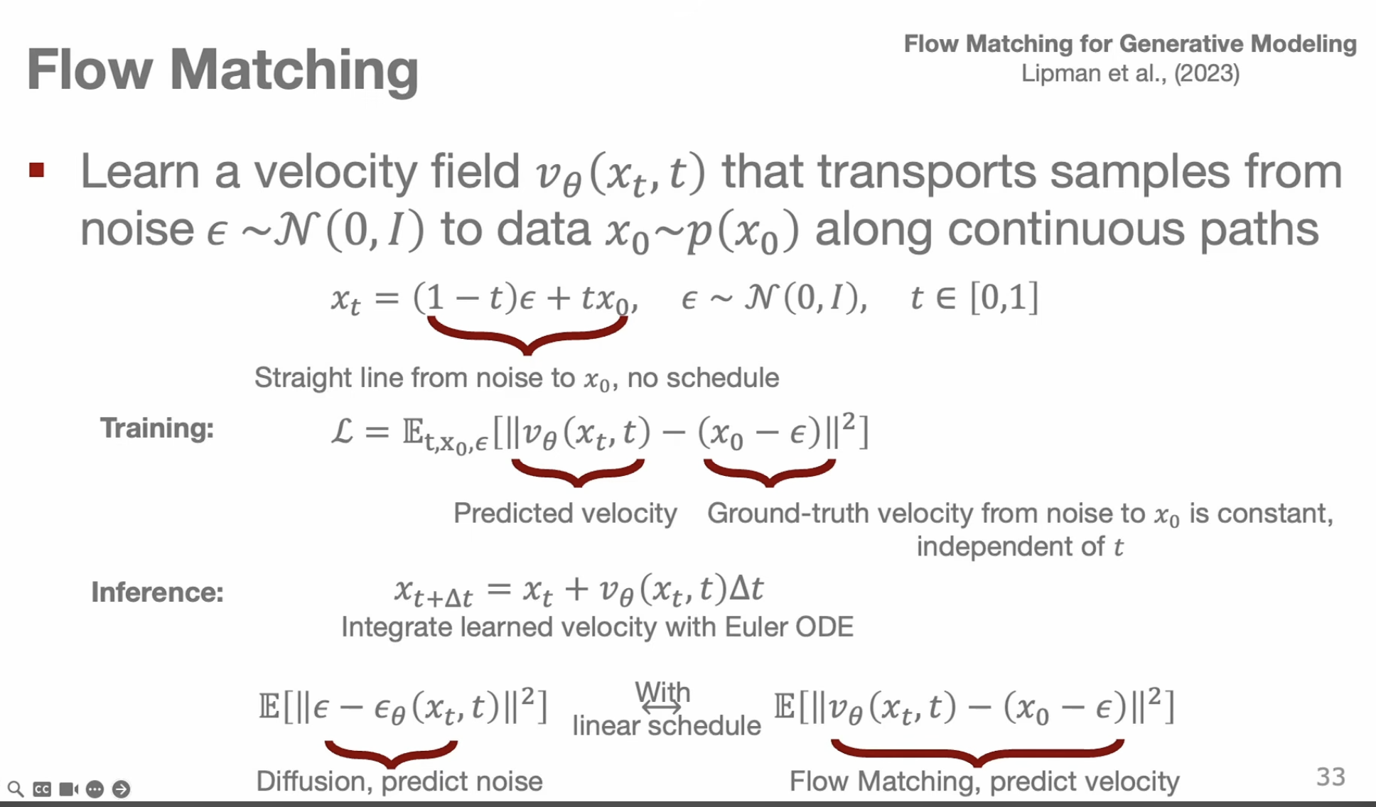
Between those, draw a path from noise to data and learn the velocity field that moves samples along it.
current point + time -> velocity directionAt inference, we start from noise and integrate the learned velocity field with an ODE solver.
So instead of predicting noise, flow matching predicts how the sample should move.
Flow matching is related to diffusion, but often easier to sample from
Diffusion and flow matching are closely related.
With certain schedules, predicting noise and predicting velocity are just different parameterizations of similar transport behavior.
But flow matching has practical advantages.
no complex noise schedule
straighter paths
fewer integration steps
The model learns a deterministic vector field from noise to data.
For robotics, fewer sampling or integration steps matter because action generation must be fast enough for control.
Flow matching Objective
Rectified flow tries to untangle crossing paths
A subtle issue appears when we randomly pair noise samples with data samples.
Straight lines between random pairs can cross.
When paths cross, the velocity field may need to point in conflicting directions at the same place.
same region in space
-> one path wants to go left
-> another path wants to go right
That forces the learned flow to curve, which makes integration slower or harder.
Rectified flow addresses this by iteratively generating better noise-data pairings using the learned flow, then retraining on those coupled pairs.
The result is straighter, less tangled transport paths.
pi0 brought flow matching into vision-language-action policies
The lecture highlights pi0 from Physical Intelligence as an important robotics example.
The core idea is to use flow matching to produce robot actions in a vision-language-action policy.
vision-language model context
+
flow-matching action generation
-> robot action outputs
The lecture describes pi0 as an early flow-matching VLA, and notes that this style has become a common default for many modern VLAs.
One technical detail: instead of sampling flow time uniformly, pi0 samples more from harder, noisier time regions using a shifted beta distribution.
That focuses training on places where action prediction needs to do more work.
The lecture's big picture is a ladder of generative policy tools
The story starts from one robotics problem:
robot behavior is multimodal
MSE deterministic policies average modes
averaging modes can fail
Then the lecture builds a ladder of generative tools.
Autoencoders: learn compressed latent structure
VAEs: make the latent space sampleable
VQ-VAEs: turn continuous signals into discrete tokens
Diffusion: generate by iterative denoising
Diffusion Policy: denoise robot action sequences
Flow Matching: learn direct velocity paths from noise to data
Rectified Flow: straighten those paths further
The main robotics takeaway:
generative models are not just for images;
they are becoming the machinery behind modern robot policies.